Imgtools - manipulate Tk photo images

The math behind image transformations

On this page we present some of the math behind image transformations.

It is by no means a complete guide on image processing. It is just a collection of some aspects that were not obvious to figure out. For my own reference and for everyone interested in the topic.

Overview
Rotation: Size of destination image
Roatation and coordinate translation
Interpolation

Overview

Very short overview how scaling and rotating images is done:

Determine the size of the destination image
Calculate values for each pixel of the destination image:
1. Apply coordinate translation, i.e. find out the position of the destination pixel relative to the source image.
2. Calculate the values for the destination pixel, interpolating from the surrounding source pixels

Top

Rotation: Size of destination image

When rotating an image, the size of the destination image is not given. There are different approaches to determine that size. We are going to have a closer look at three of them (those available in imgtools), but there are yet other approaches not mentioned here.

Top

Keep size

Make the destination image the same size as the original one. Unless the angle of rotation is a multiple of 180°, there will be empty areas in the resulting image and, at the same time, not all of the source image will be visible.

From the mathematical point of view, this is the simplest variant for sure. There's nothing to calculate!

Top

No clipping

With this approach, we make the destination image large enough to contain all of the source image. This implies that the blank areas can become a considerable portion of the image.

This rotation method looks like this:

drawing on finding size of destination image

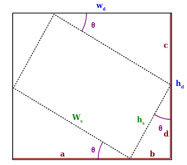
The dashed rectangle represents the rotated source image, the outer one is our destination image. θ is the angle of rotation, $w_{s}$ and $h_{s}$ are the width and height of the source image respectively. $w_{d}$ and $h_{d}$ are the sizes of the destination image - the sizes we need to calculate.

Let's see how we can calculate them:

$\begin{matrix} \underset{̲}{Calculate a, b, c and d :} \\ a = w_{s} \cos (θ) \\ b = h_{s} \sin (θ) \\ c = w_{s} \sin (θ) \\ d = h_{s} \cos (θ) \\ \underset{̲}{Now for w_{d} and h_{d} :} \\ w_{d} = a + b \\ w_{d} = w_{s} \cos (θ) + h_{s} \sin (θ) \\ h_{d} = c + d \\ h_{d} = w_{s} \sin (θ) + h_{s} \cos (θ) \end{matrix}$

There is a problem with the formula above, though: it is valid only for the interval 0° ≤ θ ≤ 90°. For greather values of θ we get slightly different formulas (the derivation of these formulae is left as an excercise for the reader :-)):

$\begin{matrix} \underset{̲}{For 90° \leq θ \leq 180°} \\ w_{d} = w_{s} (- \cos (θ)) + h_{s} \sin (θ) \\ h_{d} = w_{s} \sin (θ) + h_{s} (- \cos (θ)) \\ \underset{̲}{For 180° \leq θ \leq 270°} \\ w_{d} = w_{s} (- \cos (θ)) + h_{s} (- \sin (θ)) \\ h_{d} = w_{s} (- \sin (θ)) + h_{s} (- \cos (θ)) \\ \underset{̲}{For 270° \leq θ \leq 360°} \\ w_{d} = w_{s} \cos (θ) + h_{s} (- \sin (θ)) \\ h_{d} = w_{s} (- \sin (θ)) + h_{s} \cos (θ) \end{matrix}$

The difference between the formulae is only in the negation of the sin() and cos() values for some cases. Negation occurs exactly in those intervals where the corresponding function is negative. This means that we always get positive values for +/-sin(θ) and +/-cos(θ), which is handy, since negative distances are kinda hard to handle ;-).

It also means that we can derive a one-for-all formula:

$\begin{matrix} w_{d} = w_{s} | \cos (θ) | + h_{s} | \sin (θ) | \\ h_{d} = w_{s} | \sin (θ) | + h_{s} | \cos (θ) | \end{matrix}$

Top

No blank areas

Clip away all blank areas: make the the destination image small enough so there are no blank areas, yet try to make the destination image as large as possible. For angles of rotation that are not a multiple of 90°, portions of the source image will not be visible in the destination image.

This means that we have to inscribe a rectangle into the rotated source, such that each of its corners touches a side of the source rectangle.

All clipping size drawing

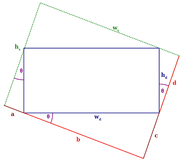
The image above shows the rotated source rectangle (green, dashed lines) and the destination rectangle we have to calculate (blue lines). $w_{s}$ and $h_{s}$ are the width and height of the source image, $w_{d}$ and $h_{d}$ are the dimensions of the destination image. a, b, c and d are distances needed in the equations below.

And here's some math!

$\begin{matrix} \underset{̲}{a, b, c and d are:} \\ a = h_{d} \sin (θ) \\ b = w_{d} \cos (θ) \\ c = w_{d} \sin (θ) \\ d = h_{d} \cos (θ) \\ \underset{̲}{We have:} \\ {\begin{matrix} w_{s} = a + b \\ h_{s} = c + d \end{matrix} \\ {\begin{matrix} w_{s} = h_{d} \sin (θ) + w_{d} \cos (θ) \\ h_{s} = w_{d} \sin (θ) + h_{d} \cos (θ) \end{matrix} \\ {\begin{matrix} w_{d} \cos (θ) = w_{s} - h_{d} \sin (θ) \\ h_{d} \cos (θ) = h_{s} - w_{d} \sin (θ) \end{matrix} \\ {\begin{matrix} w_{d} = \frac{w_{s}}{\cos (θ)} - h_{d} \frac{\sin (θ)}{\cos (θ)} \\ h_{d} = \frac{h_{s}}{\cos (θ)} - w_{d} \frac{\sin (θ)}{\cos (θ)} \end{matrix} \\ \underset{̲}{In each equation substitute w_{d} or h_{d} from the other} \\ {\begin{matrix} w_{d} = \frac{w_{s}}{\cos (θ)} - (\frac{h_{s}}{\cos (θ)} - w_{d} \frac{\sin (θ)}{\cos (θ)}) \frac{\sin (θ)}{\cos (θ)} \\ h_{d} = \frac{h_{s}}{\cos (θ)} - (\frac{w_{s}}{\cos (θ)} - h_{d} \frac{\sin (θ)}{\cos (θ)}) \frac{\sin (θ)}{\cos (θ)} \end{matrix} \\ {\begin{matrix} w_{d} - w_{d} \frac{\sin^{2} (θ)}{\cos^{2} (θ)} = \frac{w_{s}}{\cos (θ)} - h_{s} \frac{\sin (θ)}{\cos^{2} (θ)} \\ h_{d} - h_{d} \frac{\sin^{2} (θ)}{\cos^{2} (θ)} = \frac{h_{s}}{\cos (θ)} - w_{s} \frac{\sin (θ)}{\cos^{2} (θ)} \end{matrix} \\ {\begin{matrix} w_{d} \frac{\cos^{2} (θ) - \sin^{2} (θ)}{\cos^{2} (θ)} = \frac{w_{s} \cos (θ) - h_{s} \sin (θ)}{\cos^{2} (θ)} \\ h_{d} \frac{\cos^{2} (θ) - \sin^{2} (θ)}{\cos^{2} (θ)} = \frac{h_{s} \cos (θ) - w_{s} \sin (θ)}{\cos^{2} (θ)} \end{matrix} \\ \underset{̲}{With:} \cos^{2} (α) - \sin^{2} (α) = \cos (2 α) \\ {\begin{matrix} w_{d} = \frac{w_{s} \cos (θ) - h_{s} \sin (θ)}{\cos^{2} (θ)} \cdot \frac{\cos^{2} (θ)}{\cos (2 θ)} \\ h_{d} = \frac{h_{s} \cos (θ) - w_{s} \sin (θ)}{\cos^{2} (θ)} \cdot \frac{\cos^{2} (θ)}{\cos (2 θ)} \end{matrix} \\ {\begin{matrix} w_{d} = \frac{w_{s} \cos (θ) - h_{s} \sin (θ)}{\cos (2 θ)} \\ h_{d} = \frac{h_{s} \cos (θ) - w_{s} \sin (θ)}{\cos (2 θ)} \end{matrix} \end{matrix}$

As for the "no clipping" method, these formulas are valid only in the interval [0°, 90°]. To find a formula that's valid for all angles, we can figure out the other three, just as we did above, and then derive the "grand equation". Long story short, here it is:

$\begin{matrix} w_{d} = \frac{w_{s} | \cos (θ) | - h_{s} | \sin (θ) |}{\cos (2 θ)} \\ h_{d} = \frac{h_{s} | \cos (θ) | - w_{s} | \sin (θ) |}{\cos (2 θ)} \end{matrix}$

They even look similar to the "no clipping" ones, they must be correct, right?

Uhm, let's try it out. Say we have a source image of size 800x600, and we rotate it by 10°. We get a destination image of 728x481 (rounded values) - looks good.

Another try: same image, but this time we rotate it by 40°. Ouch! The result is 1308 by -314. A negative height can't be right! And the width is way too large - not good either. So what's wrong?

We didn't say so, but we assumed that there always is a rectangle that fits into our rotated source and touches its sides with all four corners. This assumption, alas, is wrong.

All clipping size drawing 2

As we can see from the graphic, the destination image gets narrower with growing angle. At some point, our destination rectangle will be just a line that goes from one corner of the source to the opposite one. Past that point, there's no way to draw a rectangle that fits our requirements. If we keep rotating, at some point we will get a valid result again.

The limits for valid results are the angles formed by the diagonal of the source rectangle and its sides. For 0° ≤ θ ≤ 90° our formulas give valid results if:

$\begin{matrix} θ < \arctan (\frac{a}{b}) \lor θ > \arctan (\frac{b}{a}) \\ (\lor means "or" ) \\ Where a is the smaller value of w_{s} and h_{s} \\ and b is the larger value of w_{s} and h_{s} \end{matrix}$

Obvously, the requirement that destination touches source with all four corneres does not work - looks like we need to take another approach. What if only two corners of the destination image must touch source edges and the other two must be inside it? With that we face another problem, though: we won't get a unique result. For any combination of width, height and angle, there is an infinite number of rectangles that meet our requirements.

If we add the condition that the area of our destination image must be maximised, we might get a good result. This requirement makes perfect sense - after all we want to keep as much as possible of the original image!

As a first step we need to find a way to express $h_{d}$ in terms of $w_{d}$ (it could be the other way around as well). We begin with a graphical representation of the problem:

All clipping size drawing 3

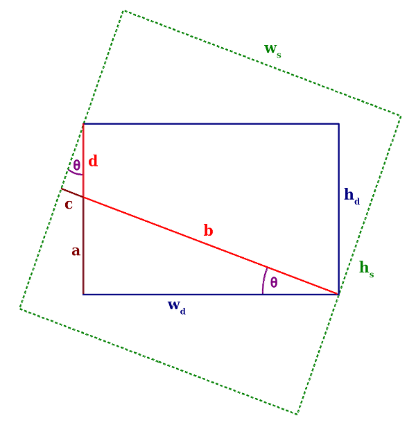
We can see that the destination rectangle must touch the longer sides of source. If it touches the shorter sides, it will not be completely inscribed in source. This means that what we are going to find out next, is valid only if $w_{s}$ < $h_{s}$ . As usual, for this first step, we consider the interval 0° ≤ θ ≤ 90° for the angle.

$\begin{matrix} \underset{̲}{The distances a, b, c and d are:} \\ a = w_{d} \tan (θ) = w_{d} \frac{\sin (θ)}{\cos (θ)} \\ b = \frac{w_{d}}{\cos (θ)} \\ c = w_{s} - b = w_{s} - \frac{w_{d}}{\cos (θ)} \\ d = \frac{c}{\sin (θ)} = (w_{s} - \frac{w_{d}}{\cos (θ)}) \cdot \frac{1}{\sin (θ)} = \frac{w_{s}}{\sin (θ)} - \frac{w_{d}}{\sin (θ) \cos (θ)} \\ d = \frac{w_{s} \cos (θ) - w_{d}}{\sin (θ) \cos (θ)} \\ \underset{̲}{Now we can express h_{d} in terms of w_{d} :} \\ h_{d} = a + d \\ h_{d} = w_{d} \frac{\sin (θ)}{\cos (θ)} + \frac{w_{s} \cos (θ) - w_{d}}{\sin (θ) \cos (θ)} \\ h_{d} = \frac{w_{d} \sin^{2} (θ) + w_{s} \cos (θ) - w_{d}}{\sin (θ) \cos (θ)} \\ h_{d} = \frac{- w_{d} [1 - \sin^{2} (θ)] + w_{s} \cos (θ)}{\sin (θ) \cos (θ)} \\ \underset{̲}{With:} 1 - \sin^{2} (α) = \cos^{2} (α) \\ h_{d} = \frac{- w_{d} [\cos^{2} (θ)] + w_{s} \cos (θ)}{\sin (θ) \cos (θ)} \\ h_{d} = \frac{\cos (θ) (w_{s} - w_{d} \cos (θ))}{\sin (θ) \cos (θ)} \\ h_{d} = \frac{w_{s} - w_{d} \cos (θ)}{\sin (θ)} \end{matrix}$

If we repeat this operation for the other three quadrants, we can determine a formula that's valid for any value of θ:

$h_{d} = \frac{w_{s} - w_{d} | \cos (θ) |}{| \sin (θ) |}$

With that, we can express the area of the destination image as a function of $w_{d}$ . As it tunrs out, it's a quadratic function with negative a, which means it has a maximum and we can calculate the value of $w_{d}$ and $h_{d}$ at this maximum.

$\begin{matrix} Express the area of destination as a function s_{(w_{d})} \\ s = w_{d} \cdot h_{d} \\ s = w_{d} \frac{w_{s} - w_{d} | \cos (θ) |}{| \sin (θ) |} \\ s = - \frac{| \cos (θ) |}{| \sin (θ) |} {w_{d}}^{2} + \frac{w_{s}}{| \sin (θ) |} w_{d} \\ The maximum of a quadratic function can be found at: \\ x_{\max} = \frac{- b}{2 a} \\ Ergo, the width for which destination has maximal area is: \\ w_{d} = - \frac{w_{s}}{| \sin (θ) |} \cdot \frac{1}{2 (- \frac{| \cos (θ) |}{| \sin (θ) |})} \\ w_{d} = - \frac{w_{s}}{| \sin (θ) |} \cdot (- \frac{| \sin (θ) |}{2 | \cos (θ) |}) \\ w_{d} = \frac{w_{s}}{2 | \cos (θ) |} \\ This allows us to calculate h_{d} as well: \\ h_{d} = \frac{w_{s} - w_{d} | \cos (θ) |}{| \sin (θ) |} \\ h_{d} = \frac{w_{s}}{| \sin (θ) |} - \frac{w_{s}}{2 | \cos (θ) |} \cdot \frac{| \cos (θ) |}{| \sin (θ) |} \\ h_{d} = \frac{2 w_{s} - w_{s}}{2 | \sin (θ) |} \\ h_{d} = \frac{w_{s}}{2 | \sin (θ) |} \end{matrix}$

As stated before, this formula works only if $w_{s}$ < $h_{s}$ . For the case where $w_{s}$ > $h_{s}$ we get similar formulas:

$\begin{matrix} \underset{̲}{h_{d} in terms of w_{d} for h_{s} < w_{s}} \\ h_{d} = \frac{h_{s} - w_{d} | \sin (θ) |}{| \cos (θ) |} \\ \underset{̲}{This gives us:} \\ w_{d} = \frac{h_{s}}{2 | \sin (θ) |} \\ h_{d} = \frac{h_{s}}{2 | \cos (θ) |} \end{matrix}$

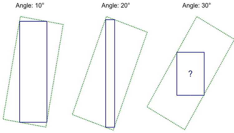
Is that it? Do these formula always give us valid results? Nope. Consider this:

All clipping size drawing 4

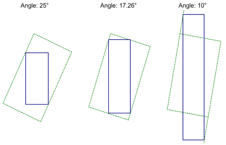
Turns out that the maximise-area approach works well if the angle is close to 45°. As we go towards 0° or 90°, at some point the destination rectangle reaches out of source!

Consider the point just before the destination image with maximised area starts becoming too large. In the example above, that's at about 17.26°. At this point, destination touches source with all four corners. Sounds familiar? Right, we've calculated that already. Looks like that effort was not vain, after all! Notice that there is another similar "turning point" somewhere between 45° and 90°, and two more in each of the other quadrants.

We are getting close to the solution for our problem. For angles between 0° and the first turning point, we well use the 4-corners approach we explored before. Between the turning points, the 2-corners-with-maximised-surface approach will give us a good result. After that, it's gonna be 4-corners again.

We have to figure out one last thing: where are these turning points?

$\begin{matrix} \underset{̲}{For w_{s} < w_{h} and 0 ° \leq θ \leq 90 ° we have:} \\ 4 corners variant: w_{d} = \frac{w_{s} \cos (θ) - h_{s} \sin (θ)}{\cos (2 θ)} \\ 2 corners variant: w_{d} = \frac{w_{s}}{2 \cos (θ)} \\ \underset{̲}{The intersection point of the two functions is:} \\ \frac{w_{s}}{2 \cos (θ)} = \frac{w_{s} \cos (θ) - h_{s} \sin (θ)}{\cos (2 θ)} \\ w_{s} \cos (2 θ) = 2 \cos (θ) (w_{s} \cos (θ) - h_{s} \sin (θ)) \\ w_{s} \cos (2 θ) = 2 w_{s} \cos^{2} (θ) - 2 h_{s} \sin (θ) \cos (θ) \\ \underset{̲}{With:} \cos (2 α) = \cos^{2} (α) - \sin^{2} (α) \\ w_{s} [\cos^{2} (θ) - \sin^{2} (θ)] = 2 w_{s} \cos^{2} (θ) - 2 h_{s} \sin (θ) \cos (θ) \\ 2 h_{s} \sin (θ) \cos (θ) = 2 w_{s} \cos^{2} (θ) - w_{s} \cos^{2} (θ) + w_{s} \sin^{2} (θ) \\ 2 h_{s} \sin (θ) \cos (θ) = w_{s} \cos^{2} (θ) + w_{s} \sin^{2} (θ) \\ \underset{̲}{With:} \cos^{2} (α) + \sin^{2} (α) = 1 \\ \underset{̲}{and:} \sin (α) \cos (α) = \frac{1}{2} \sin (2 α) \\ 2 h_{s} \cdot \frac{1}{2} \sin (2 θ) = w_{s} [\cos^{2} (θ) + \sin^{2} (θ)] \\ h_{s} \sin (2 θ) = w_{s} \cdot 1 \\ \sin (2 θ) = \frac{w_{s}}{h_{s}} \\ \underset{̲}{For any value of θ that beomes:} \\ | \sin (2 θ) | = \frac{w_{s}}{h_{s}} \\ \underset{̲}{And for w_{s} > h_{s} :} \\ | \sin (2 θ) | = \frac{h_{s}}{w_{s}} \end{matrix}$

Phew, that was some work. But we've got it now!

To sum it up: to find the dimensions for our destination image, we need first to find out on which side of those turning points we are. Depending on that, we will use either the 4-corners or the 2-corners variant. Formally, that would be:

$\begin{matrix} Let r = \frac{a}{b} \\ Where a is the shorter side, b the longer side of the source image \\ \underset{̲}{If | \sin (2 θ) | < r :} \\ w_{d} = \frac{w_{s} | \cos (θ) | - h_{s} | \sin (θ) |}{\cos (2 θ)} \\ h_{d} = \frac{h_{s} | \cos (θ) | - w_{s} | \sin (θ) |}{\cos (2 θ)} \\ \underset{̲}{If | \sin (2 θ) | \geq r and w_{s} < h_{s} :} \\ w_{d} = \frac{w_{s}}{2 | \cos (θ) |} \\ h_{d} = \frac{w_{s}}{2 | \sin (θ) |} \\ \underset{̲}{If | \sin (2 θ) | \geq r and w_{s} \geq h_{s} :} \\ w_{d} = \frac{h_{s}}{2 | \sin (θ) |} \\ h_{d} = \frac{h_{s}}{2 | \cos (θ) |} \end{matrix}$

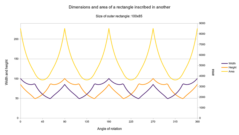
If we plot that, we get a pretty funny curve. Mountains!!

Mountains!

Top

Rotation and coordinate translation

Coordinate translation means to transform the coordinates of a point in the destination image to coordinates relative to the source image. To picture what that means, imagine to rotate the source image by θ degrees. Then lay the (not rotated) destination image over that. Now, take a needle and punch it through both images at the position we need to translate. Last, remove the needle and destination image and look where the needle punched the original image. The coordinages of that point in the source image are our translated coordinates. And it is from the source values at that point (and those near it) that we will calculate values for our destination pixel.

If we want to avoid all that needle punching and let our computer do the work instead, we need to express that in more algebraic terms. First, a drawing:

yet another drawing

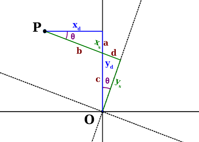
We have two sets of coordinate axes here: the continuos lines are the axes of the destination image, the dashed lines the ones of the rotated source image.

P is a point for which we know the coordinates in destination. Those coordinates are the distances $x_{d}$ and $y_{d}$ . We need to find the coordinates in terms of source, $x_{s}$ and $y_{s}$ . While the origin for both coordinate systems is the same, the axes are rotated by θ degrees. That's why the source coordinates are going to be different.

$\begin{matrix} \underset{̲}{Calculate a, b, c and d :} \\ a = x_{d} \tan (θ) = x_{d} \frac{\sin (θ)}{\cos (θ)} \\ b = \frac{x_{d}}{\cos (θ)} \\ c = y_{d} - a = y_{d} - x_{d} \frac{\sin (θ)}{\cos (θ)} \\ d = c \cdot \sin (θ) = [y_{d} - x_{d} \frac{\sin (θ)}{\cos (θ)}] \sin (θ) = y_{d} \sin (θ) - x_{d} \frac{\sin^{2} (θ)}{\cos (θ)} \\ \underset{̲}{With that we can calculate x_{s}} \\ x_{s} = b + d \\ x_{s} = \frac{x_{d}}{\cos (θ)} + y_{d} \sin (θ) - x_{d} \frac{\sin^{2} (θ)}{\cos (θ)} \\ x_{s} = \frac{x_{d} - x_{d} \sin^{2} (θ)}{\cos (θ)} + y_{d} \sin (θ) \\ x_{s} = \frac{x_{d} (1 - \sin^{2} (θ))}{\cos (θ)} + y_{d} \sin (θ) \\ \underset{̲}{With:} 1 - \sin^{2} (θ) = \cos^{2} (θ) \\ x_{s} = \frac{x_{d} \cos^{2} (θ)}{\cos (θ)} + y_{d} \sin (θ) \\ x_{s} = x_{d} \cos (θ) + y_{d} \sin (θ) \\ \underset{̲}{y_{s} is a a little simpler:} \\ y_{s} = c \cdot \cos (θ) \\ y_{s} = [y_{d} - x_{d} \frac{\sin (θ)}{\cos (θ)}] \cos (θ) \\ y_{s} = y_{d} \cos (θ) - x_{d} \sin (θ) \end{matrix}$

These equations are not quite what we want yet. You might have noticed that with those calculations our image will be rotated around the origin of the coordinate system. This means that we would rotate our image around the upper left corner, since in digital images the coordinate (0,0) refers to that corner. But... We want to rotate our image around the center!

In order to achieve this, we transform the destination coordinates to make them relative to the center of the image, apply the formula we just found and transform the result back to coordinates relative to the upper left corner.

In order to transform coordinages so they are relative to the center we must substract the distance from the pixel at (0,0) to the center of the image. Similarly, to transform back to a system relative to the top leftmost pixel, we add that distance.

At first thought, you'd probably say that this distance is half of width and height. Close, but wrong.

The center of an image is at the point that's exactly in the middle of the top leftmost and the bottom rightmost pixels.

$\begin{matrix} The coordinates of the top leftmost pixel are: (0, 0) \\ The coordinages of the bottom rightmost pixel are: (w - 1, h - 1) \\ where w and h are width and heigth. \\ The middle point C between two coordinates is: \\ C = (\frac{x 2 - x 1}{2}, \frac{y 2 - y 1}{2}) \\ In consequence, the center O of an image has coordinates: \\ O = (\frac{w - 1}{2}, \frac{h - 1}{2}) \\ Wich are, by definition, the distances of the center from the origin. \\ With that we can transform coordinates: \\ x_{dO} and y_{dO} are coordinates in destination, relative to the center: \\ x_{dO} = x_{d} - \frac{w_{d} - 1}{2} \\ y_{dO} = y_{d} - \frac{h_{d} - 1}{2} \\ Similarly, source coordinates relative to the upper left corner \\ can be calculated from source coordinates relative to the center: \\ x_{s} = x_{sO} + \frac{w_{s} - 1}{2} \\ y_{s} = y_{sO} + \frac{h_{s} - 1}{2} \\ Apply translation to the coordinates relative to the center: \\ x_{sO} = x_{dO} \cos (θ) + y_{dO} \sin (θ) \\ y_{sO} = y_{dO} \cos (θ) - x_{dO} \sin (θ) \\ Transform to coordinates relative to the upper left corner and resolve: \\ x_{s} = x_{sO} + \frac{w_{s} - 1}{2} = x_{dO} \cos (θ) + y_{dO} \sin (θ) + \frac{w_{s} - 1}{2} \\ x_{s} = (x_{d} - \frac{w_{d} - 1}{2}) \cos (θ) + (y_{d} - \frac{h_{d} - 1}{2}) \sin (θ) + \frac{w_{s} - 1}{2} \\ x_{s} = x_{d} \cos (θ) + y_{d} \sin (θ) - \frac{w_{d} - 1}{2} \cos (θ) - \frac{h_{d} - 1}{2} \sin (θ) + \frac{w_{s} - 1}{2} \\ y_{s} = y_{sO} + \frac{h_{s} - 1}{2} = y_{dO} \cos (θ) - x_{dO} \sin (θ) + \frac{h_{s} - 1}{2} \\ y_{s} = (y_{d} - \frac{h_{d} - 1}{2}) \cos (θ) - (x_{d} - \frac{w_{d} - 1}{2}) \sin (θ) + \frac{h_{s} - 1}{2} \\ y_{s} = y_{d} \cos (θ) - x_{d} \sin (θ) - \frac{h_{d} - 1}{2} \cos (θ) + \frac{w_{d} - 1}{2} \sin (θ) + \frac{h_{s} - 1}{2} \end{matrix}$

Top

Interpolation

Now we know how to translate the coordinates of a destination pixel, i.e. we know its position in the source image. Most likely that position is not going to be an integer value, which means that it is somewhere in between known data points in the source image. To get a realistic value for our destination pixel, we must interpolate from the surrounding source pixels.

There are different flavours of interpolation, with different caracteristics in quality and computing time.

The most common interpolation methods in image processing are:

(Bi-)Cubic spline interpolation (there are different sub-types, the most common is the Catmull-Rom spline)
Lanczos interpolation
Linear interpolation
Nearest neighbour

There are lots of documents about this topic on the net, so we won't go in more detail here. Here are a few pointers you might find useful or interesting:

Tutorial on image resampling
Multi-Linear interpolation [pdf]
Basics of Image Resampling and Bicubic resampling
Spline Tutorial Notes [pdf]. A lengthy document about spline interpolation in computer animation

Top

Contact | Hosting: | | Last updated: September 2017